It is only a little over a year since we released the first version of our new EBSD data processing software, AZtecCrystal, and just a few weeks since customers started using the latest major release, AZtecCrystal v2.0. This latest version has many exciting new features, such as a Classification Tool that uses machine learning to help you to partition datasets into distinct classes (such as recrystallised and deformed fractions, or to separate martensite from ferrite) and a Materials Properties viewing mode that can convert your crystallographic orientations into elastic property data such as the Young’s Modulus. Many of these headline features are highlighted on the AZtecCrystal webpage, and the interactive video on that page lets you see how they work in practice.

However, the ongoing development of AZtecCrystal has enabled us to add lots of additional, less-prominent functionality into the software and I want to use this blog to bring these to your attention. In particular, I want to introduce the use of templates in the software, the new boundary statistics viewer and to show how you can use AZtecCrystal to estimate the parent grain size in relevant datasets.

Templates – making your life easier

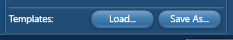
It is common that we want to perform repeated tasks when processing EBSD data. This might mean that we always want to plot the same few maps or to clean our data using a specific recipe. We now have template functionality in AZtecCrystal that enables us to store templates from any viewing mode within the software. This includes (but is not limited to) defining a clean-up recipe, specifying the grain size measurement parameters, or storing the settings for any map, pole figure or orientation distribution function (ODF) display. The process is simple: once a particular process or display has been defined, you simply click on the “Save As…” button that is located at the bottom of the relevant settings panel and give the template an appropriate name:

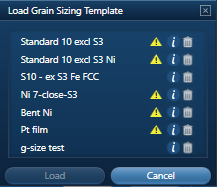
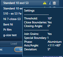
Then, when you want to reuse that template, you can just load it from the list of available stored templates. However, the system is smart enough to know when there may be conflict issues in any given template – for example if a twin boundary has been defined for a specific phase, but that phase is not present in the current dataset. In such cases the template will be marked with a warning triangle. In the case below (during the analysis of data collected from a duplex steel sample), a number of grain size measurement templates display warning triangles (left image). Clicking on the adjacent information symbol for the first template in the list shows us that it includes the exclusion of a twin boundary for a phase (aluminium) that is not present in the current dataset (right image):

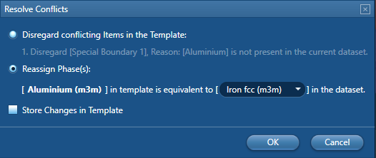
You can still use such templates, but the system will ask whether you want to disregard the conflict (in which case, in this example, it will not exclude the twin boundary in the grain size measurement) or whether you want to reassign the phase – here we can apply the twin law to the Iron FCC phase in our dataset and have the option to update the template information to use this new phase in any subsequent application:

I find that I am using the templates frequently in my analysis of EBSD data and it really does make my life easier. As a final note, remember that you can also combine multiple templates using the Batch functionality (via the Tools dropdown menu), but that is a topic for another blog.

Uncovering precise boundary statistics

Boundaries are critical features in any microstructure and EBSD is a uniquely powerful technique for examining them, providing information about their crystallographic and physical properties. We have had the ability to examine boundary disorientations and associated rotation axes in AZtecCrystal since early in 2020 (available in the Boundaries viewing mode), but this latest release includes a more comprehensive boundary statistics tool. Here we can study the relative lengths of all types of boundaries in our samples and, importantly, it is very easy to use. The statistics will always reflect the currently selected map, so if there are particular boundary types that you are interested in (such as specific disorientation ranges, twin boundaries or phase boundaries), then you simply need to make sure that the current map has those boundaries displayed.

In the case below, we are looking at the relative lengths of boundaries across different disorientation ranges for both phases in a duplex steel sample:

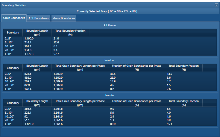
For the statistics on other boundary types (such as coincident site lattice or phase boundaries), these will appear on separate tabs in the display, but only if those boundaries are plotted in the current map. If there is no relevant tab, that is because the boundaries are not displayed in the map. It’s also important to note that AZtecCrystal calculates the true lengths of the boundaries, taking into account the orientation of the boundary trace. Without this, boundaries that are oriented at 45° to the horizontal would have boundary lengths a factor of √2 longer than their true lengths due to the pixelated nature of EBSD maps. AZtecCrystal uses some well-established correction factors to determine 2D lengths in digitised space (see, for example, B. Verner, Pattern Recognition Letters 12 (1991) 671—682), so you can be confident in the results shown in these tables. And remember, right mouse clicking on the table will allow you to export all the results to a text file format.

Measuring parent grain sizes

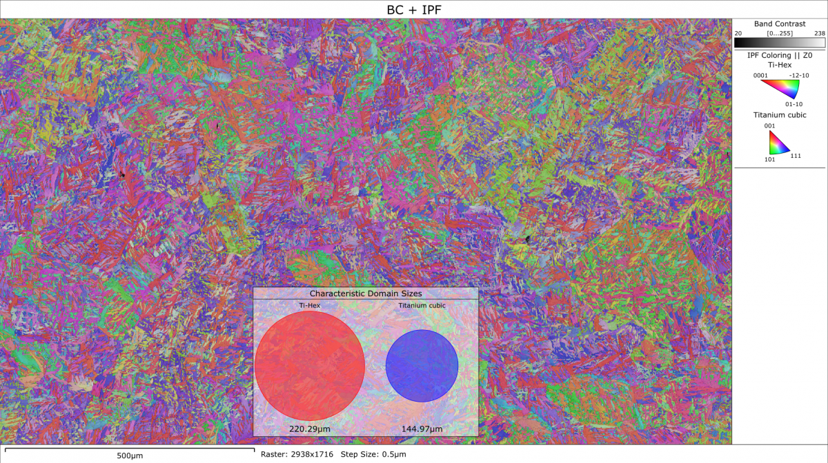
We often hear from customers that they are interested in determining parent grain sizes (for example, prior austenite grains in steels or prior Beta grains in Ti alloys), and know that there are plenty of research groups working on developing new algorithms to reconstruct parent microstructures. However, in AZtecCrystal we have implemented a new tool that quickly and effectively can give you an estimate of the parent grain size. This uses an elegant concept published a few years ago called the Distance Disorientation Function (DDF) – see Morales-Rivas et al., Journal of Materials Science (2015) 50:258–267. The principles of the DDF are quite simple – the daughter grains (or variants) that originated from a single parent grain are likely to have specific, non-random orientation relationships between them, and this means that if you measure the frequency distribution of disorientation angles between points that are separated by only short distances, then that distribution will reflect the abundance of “special” disorientations between the different variants. However, increasing the distance between measurements will gradually reduce the influence of these special disorientations until, at a certain distance, the disorientation distribution will be indistinguishable from that of randomly selected pairs of points from the whole dataset. This distance is essentially reflecting the average size of the parent grains in the microstructure; AZtecCrystal calculates this size automatically in the Boundaries viewing mode and calls it the “Characteristic Domain Size” (CDS).

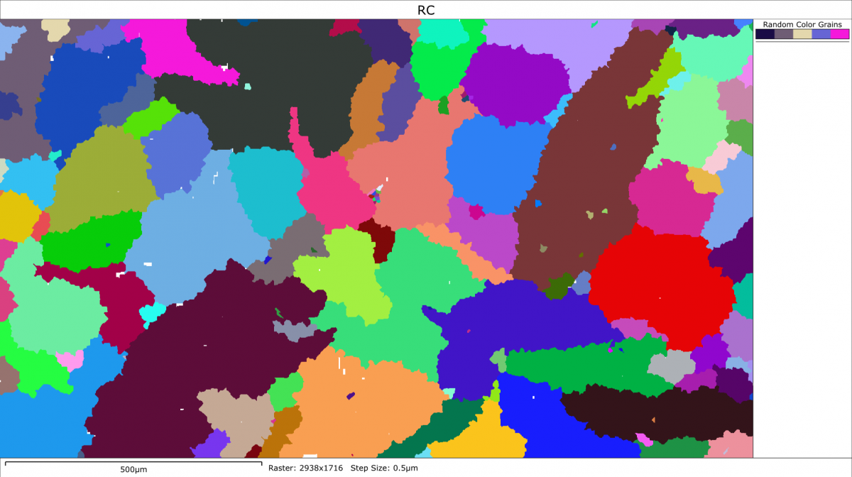
How well does it work? The first key point is that you need (a) enough parent grains within your map (probably >50 to ensure success) and (b) enough boundary measurements to get a reliable result – I would recommend 100,000 (up from the default value of 10,000). When testing it on a variety of microstructures, the results visually match the parent grain sizes very well. For example, the following orientation map was collected from an additively-manufactured Ti64 alloy. There is about 1-2% of retained beta-Ti, but the calculated CDS from the alpha-Ti is measured as 220 mm, compared to a directly measured (area-weighted) mean grain size of 12 mm. Visually this looks to fit the parent grains very well (see the red circle on the map), but in this dataset we can use another trick: by deleting the alpha-Ti from the dataset and iteratively “growing” the remaining beta-Ti grains until they coalesce, we can reconstruct the original high temperature microstructure (of course this assumes that the many retained beta-Ti grains maintain the original orientation of the parent grains). The resulting grain map is shown below the orientation map, and the beta-Ti grain size here is measured as 201 mm, within 10% of the CDS value of 220 mm.

So it would seem that the DDF concept works quite well, and we can use it to give an initial estimation of parent grain sizes in a range of different materials. I would not compare it to some of the more sophisticated parent-grain reconstruction algorithms that have been published in recent years, but if you want a quick tool to evaluate the prior microstructural domains, then give it a go!

So that’s all in this initial AZtecCrystal Tips and Tricks blog. Hopefully we’ll have another blog covering a few more of the hidden tools in AZtecCrystal in the coming months, but don’t forget that there are many useful videos in the Learning Hub on our website, both under the Tips and Tricks videos and the Tutorial and Demo videos. In the meantime, don’t hesitate to get in touch with us if you have any questions or comments regarding our AZtecCrystal software.

Dr Pat Trimby

EBSD Product Manager