产品
FIB-SEM
Nanomanipulators
OmniProbeOmniProbe Cryo软件
AZtec3DAZtecFeatureAZtec LayerProbeTEM
Hardware
EDSUltim MaxXploreImaging
软件
AZtecTEM
 牛津仪器集团成员

16th June 2021 | Author: Dr Pat Trimby
One of the great things about my role as EBSD Product Manager is that I am always learning new things about the EBSD technique and the wider field of electron and ion microscopy. Recently, I was fortunate to be invited as a speaker at an excellent microscopy school, organised by McMaster University in Canada. There were many fascinating talks, covering topics ranging from energy dispersive X-ray spectrometry (EDS) to the ongoing advances in the field of focused ion beam (FIB) microscopy. However, of particular interest to me was a presentation given by Dr. Joe Michael from Sandia National Laboratories in the US, titled “Introduction to EBSD: Current Issues in Data Presentation”. As one of the outstanding EBSD scientists over the past 3 decades, Joe’s talks are always worth listening to and will invariably deliver a few nuggets of information that are worth hoarding for future use, and this presentation was no exception.
In his role as an editor with one of the prominent microscopy journals, Joe was lamenting about some poor practices in EBSD data processing that are frequently on display in the manuscripts he reviews. This started me thinking about how we can help our customers to establish good habits when using our software, AZtecCrystal. We are on the cusp of releasing AZtecCrystal version 2.1 and are continuing our rapid development plans with a view to incorporating additional new functionality later in the year. However, sometimes it is beneficial to step back from the exciting new features and instead focus on minor tweaks that can make a big impact to the everyday processing of EBSD data. It is just some of those smaller changes that I want to focus on in this post; perhaps drawing these to your attention will help improve your EBSD data analysis routines and might even please Joe if one of your manuscripts passes across his desk.
Rarely do we achieve 100% perfect data with EBSD. In fact, most real-world samples have surface blemishes, voids, cracks and perhaps some surface topography that represent areas that should never give an indexed solution in an EBSD scan. If I see an EBSD map with 100% indexing, then I am immediately suspicious: either the data have been cleaned, or there are likely to be some false data present. In most EBSD scans of polycrystalline materials, we will see points along grain boundaries that have not been successfully indexed. This is usually due to the superposition of diffraction patterns from the crystallites on either side. In order for us to measure reliably a number of important parameters such as boundary properties and grain size, we almost always need to perform at least some data cleaning.
There are 2 important messages here:
As an example, recently I was looking at a published paper showing EBSD data in a particularly interesting research field and was surprised to see 100% indexing in all the displayed orientation maps. This was despite the fact that I know from personal experience that the material in question is exceptionally challenging to analyse using EBSD. A closer inspection suggested that the EBSD maps had been aggressively cleaned, to the extent that many of the features (such as grain shapes and boundary traces) looked very artificial. I won’t reference the work, for obvious reasons, but the lack of any mention of data cleaning in the text made me dismiss the scientific value of the paper. The take home message is that if you are not transparent about how you have processed your data, then you can’t be surprised if others to trust your interpretations.
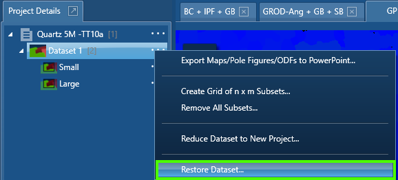
In AZtecCrystal, we do offer a whole host of data clean up tools: these include an “Auto Clean” routine, isolated error removal, extrapolation of solutions into non-indexed pixels, pseudo-symmetric error removal and, in the upcoming 2.1 version, a Kuwahara filter to reduce some orientation noise. All of these tools can be powerful, but all should be applied with care. If you want to revert back to the original raw data, this is always possible, either via the Clean Up viewing mode or directly on the Project Details panel – right click on the relevant dataset or press the associated “…” icon, and you will see the “Restore Dataset” option:
If you want to see the data processing history (even if you have been sent a pre-cleaned dataset), this will be visible in the Project Information. You can view this simply by clicking on the Project name in the Project Details panel:
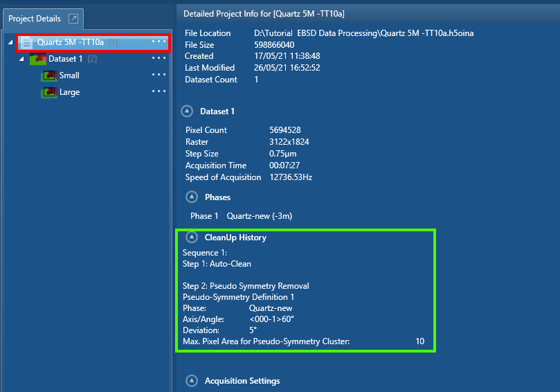
This example shows the data clean up steps that I performed when processing a geological dataset for the recent AZtecCrystal Tutorial, which you can view here.
EBSD is, on the face of it, the perfect technique to measure grain sizes in materials; it is fast, has excellent spatial resolution and is fully quantitative. However, as various Round Robin exercises have demonstrated in the past, different laboratories can get wildly different grain size measurements from identical samples. The key factor, in all cases, is to ensure that the original data is of the highest quality possible – there is no point in having high hit rates (the percentage of analysis points indexed) if a significant fraction of those points will have incorrect phases or orientations. Take a little longer over the measurements to ensure that the data are the best quality that you have time for. Of course, for a simple metal or alloy sample, it should be possible to analyse at the fastest speeds delivered by your detector – such as >4500 patterns per second with the Symmetry S2 detector – confident that you can achieve close to 100% indexing with virtually zero errors. However, this will not be the case for a cold deformed steel or a complex geological sample. Sometimes slower is better.
Once you have your data, again you will need to carefully perform the necessary clean-up steps ensuring that you only do what is required to get valid, representative grain size data.
At this point, it is worth mentioning some of the EBSD grain size standards, such as ISO 13067 and ASTM E2627, as these provide guidance on how to perform EBSD experiments for grain size measurements. The 2 main standards can be summarised as follows:
| Standard | Minimum no. of pixels per grain | Maximum % modified during clean up | Minimum number of grains |
| ISO 13067 | 10 | 5% | 500-100 |
| ASTM E2627 | 100 | 10% | 500 |
These are good starting points for any effective grain size analysis. I would tend to use the ISO standard more commonly, as I feel that the 100 pixel minimum specified by the ASTM standard results in significant oversampling of the microstructure, with minimal benefit in terms of the resulting grain size accuracy.
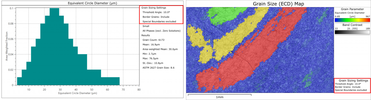
Whenever reporting grain size results (or any grain-related data display), you should always report the settings used for the grain detection. In the upcoming AZtecCrystal release, we have added this information to the legend associated with any grain-related data export, as highlighted in the following examples:
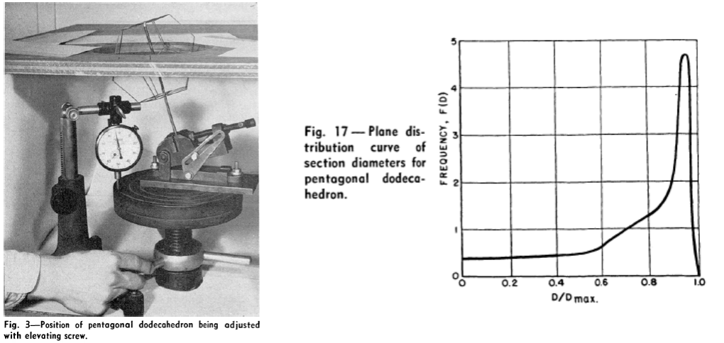
Perhaps the most important aspect of grain size measurement and the display of grain size results relates to the grain size histogram. In his presentation, Joe was particularly vocal in his dismay at the misinterpretation of this histogram, as this is not representing the grain size distribution, but is a result of the 2D sectioning of a 3D microstructure. He referred to a paper that I had not encountered before, written back in 1953 by F.C. Hull and W.J. Houk – “Statistical Grain Structure Studies: Plane Distribution Curves of Regular Polyhedrons” (JOM 5, p 565-572). In this work, the authors set up an experimental rig to measure the shape and size of the intersection between various 3D grain shapes and a 2D plane, with differing heights, as shown below. The results are fascinating, with the distribution of the measured grain diameters illustrating how we must be careful with our interpretations of the grain “size” histograms. Remember, the histogram below is the “size distribution” you would see when the true grain size is completely uniform in 3D (in this case for a pentagonal dodecahedron grain shape):
So, in summary, EBSD is great at measuring the average grain size (albeit requiring 3D stereological corrections) but is not a good technique for measuring the grain size distributions, unless you are prepared to perform 3D EBSD – but that’s a topic for another day. And, of course, this shows that we can all keep learning, even from research carried out almost 70 years ago!
We send out monthly newsletters keeping you up to date with our latest developments such as webinars, new application notes and product updates.

© 牛津仪器 2026
 公安机关备案号31010402003473