I really hope that you’ve found my last two blogs on how to optimise AZtecFeature useful – we looked at Thresholding – the process we use to identify where features are and where one ends and the next one begins in the first one – and Classification – the way in which groups of particles within a population can be gathered together in the second.  Both of these are very important parts of the particle or feature analysis process.  Today, we’re going to move on and consider how to choose an appropriate magnification for our large area feature analysis runs. 

We have the ability to look at all sorts of different sample types with AZtecFeature – particles, inclusions, and solid samples to name a few.  One of the key parameters that we have to decide upon when determining our analytical conditions for an AZtecFeature analysis is what magnification to use.  This is a really important parameter for a number of reasons.  Firstly, it plays a large part in determining what the smallest object that we can analyse is – the higher the magnification the smaller feature size we can analyse.  Secondly, it has a very large effect on how long our analysis will take when we perform a large area run:  If we wish to analyse a certain area of a sample, then, at a higher magnification we will need more fields of view to cover that area than we would at lower magnification.  This means more stage moves and more image acquisitions – all of which take time – and that time multiplies up very quickly as the area that we analyse gets larger or the magnification increases.  As such, particularly in time sensitive applications, there is often a desire to work at the lowest magnification possible.

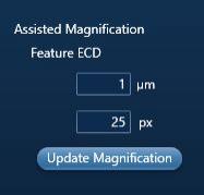
It can sometimes be difficult to know what magnification is appropriate for the sample you’re looking at.  If good quality measurements are required from each particle, I would normally recommend aiming for around 25 pixels in the smallest particle that you’re interested in.  AZtecFeature has a function called Assisted Magnification that can help with working out what magnification that corresponds to.  By entering the size of the smallest feature that you’re interested in and how many pixels you want a feature of that size to contain, AZtec will calculate, taking into account the resolution you are working at and your particular microscope calibration, what magnification is required in order to achieve that number of pixels in a feature of that size and set the microscope accordingly.

The general advice I always give when determining magnification is to set it up so that you can accurately image the smallest feature that you are interested in.  If the features in the sample are all approximately the same size then this works well as the magnification is effectively optimised for all features.  However, a problem can occur when working with samples that have a range of feature sizes.  If the magnification is optimised for the larger features then, whilst the run will be quick it will also be unable to resolve the smallest features.  If, on the other hand, the magnification is optimised for the smallest features (as recommended above!) then the larger features may well be broken by the field boundaries.

This situation can make it very difficult to decide upon an appropriate magnification to use.

AZtecFeature includes another piece of functionality to overcome this issue.  When the large area analysis is performed with a small field overlap it is able to reconstruct features that have been broken by field boundaries over multiple fields.  You can see an example of this below.

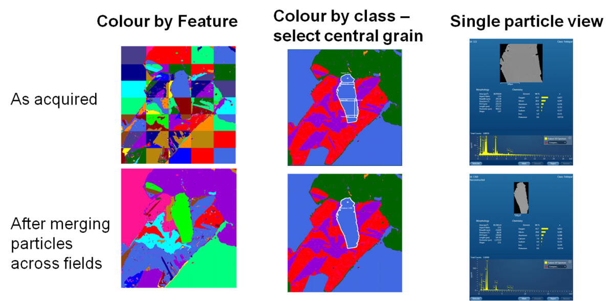
The top left image shows a dataset as acquired.  Here, we have randomly coloured each feature as acquired – you can see from the checkerboard pattern where features have been broken by field images.  When that same image is viewed in terms of classification – in the top middle image – it looks OK at first glance.  However, the broken grains are evident when you start selecting them.  In fact, the large grain coloured blue at the centre of the field of view is made up on 5 separate acquisitions – the image on the top left shows the details for the middle part of the grain.  This has significant implications for the dataset.  Firstly, our number of grains will be wrong as we have multiple acquisitions for what we know to, in reality, be one grain.  Secondly, our morphology measurements will be skewed towards smaller grain sizes and thirdly, the compositions that we calculate will be affected by being from multiple small areas instead of a larger area.

The bottom row of images shows the same data after AZtecFeature’s reconstruction algorithm has been run.  Now, the bottom left image makes sense – we don’t see the checkerboard pattern anymore even though we are using the same colouring scheme.  This is confirmed in the bottom middle image – the classification remains correct and, when we select the central grain we now get a morphology for it which is correct and a recalculated composition based upon the component parts.

So, as we’ve seen, magnification is a very important parameter for us to set correctly.  By using both assisted magnification and reconstruction for larger features, AZtecFeature allows you to be confident that you are getting the right results from your feature analysis – regardless of feature size.

Are you struggling to get started with your particle analysis? Book a demo now to experience the power of AZtecFeature.

Dr Matt Hiscock

Head of Product Science